stepwise: StepWise Monte Carlo for modeling small RNA & protein motifs
Application purpose
The stepwise monte carlo code is intended to give three-dimensional de novo models of RNA and protein motifs, with the prospect of reaching high accuracy. It differs from fragment assembly approaches in not relying on the database of known structures, and therefore is appropriate for problems that need to be modeled 'ab initio'.
Stepwise monte carlo is slower than fragment-based approaches, but appears comparable in speed to KIC-based loop modeling, and is much faster and easier to run than the original stepwise enumeration methods. The code has been written in a modular fashion so as to allow its testing to new problems by Rosetta developers, including non-natural backbones, cyclic peptides/nucleotides, disulfide-bonded proteins, and ligand docking.
A useful 20-minute description of the basis and conceptual framework of stepwise monte carlo is available here:
Slides are also available in keynote format here.
Algorithm
This monte carlo minimization method builds up models by moves that involve sampling and minimization of single residues, what we've previously termed a 'stepwise ansatz'. Unlike other modes of Rosetta, moves include the deletion and addition of single residues. Because these moves are concentrated at termini, they are accepted frequently and allow deep optimization of an all-atom energy function. For some problems, poses can also be split and merged, and separate chains can be docked or undocked. This same stepwise framework and application also reimplements enumerative sampling, following a recursion relation described previously (the 'stepwise assembly' method); in future releases, the older code will be removed.
Options
A full accounting of options you may want to use is also available.
Commonly used options
-s                                  Input file(s). For motifs that connect multiple helices like two- or three-way junctions, one may
                                    consider providing helices as distinct input files; the algorithm will allow them to move relative to
                                    each other.
-in:fasta                           Fasta-formatted sequence file. [FileVector]
-extra_minimize_res                 List of residues (either Rosetta numbering or resnum-chain (A:1-5) which may be minimized despite
                                    being provided as part of the 'starting structure'
-terminal_res                       List of residues (either Rosetta numbering or resnum-chain (A:1-5) which are the terminal residues of
                                    the starting structure(s) provided
-motif_mode                         If provided, Rosetta will automatically compute -extra_minimize_res and -terminal_res
-chemical::enlarge_H_lj             Use a physically realistic H LJ radius, preventing collapse of RNA helices.
-out:file:silent                    Name of output file [scores and torsions, compressed format]. default="default.out" [String]
-in:native                          Native PDB filename. [File].
-out:nstruct                        Number of models to make. default: 1. [Integer]
-score:weights                      Scoring function (weights file) to use. The official 'best practice' at the moment is to use
                                    -score:weights stepwise/rna/rna_res_level_energy4.wts -restore_talaris_behavior; currently in development
                                    is stepwise/rna/rna_res_level_energy7beta.wts, which does not require -restore_talaris_behavior.

Useful options
--------------
-monte_carlo:submotif_frequency     Adjust the frequency of 'submotif moves' (taken from a database of native structures). When
                                    benchmarking, it can be useful to set this to 0.0 to ensure no part of the target loop is being built
                                    from a native.
-cycles                             Number of Monte Carlo cycles.[default 50]. [Integer]
Limitations
This method is not guaranteed to give an exhaustive search of a physically realistic subspace of RNA/protein conformations, which was a nice feature of the original stepwise assembly work. Instead, like nearly all Rosetta protocols (KIC modeling, etc.) the sampling can return different solutions starting from different starting seeds, and you should check for convergence from independent runs.
The method is acutely sensitive to the assumed energy function. This is in contrast to other Rosetta protocols that either transit through low-resolution ('centroid') stages or make use of database fragments; both strategies 'regularize' the search but preclude solution of problems in which low-resolution energy functions are not trustworthy or the fragment database is too sparse.
The method computes loop closure (
loop_close) energies based on a simple Gaussian chain model of uninstantiated loops. While this energy function can handle cycles of loops, it fails on pose collections that have nested loop cycles, and so those are avoided by default instepwise.The method is intended to obey detailed balance, albeit on a perturbed energy landscape where each conformation's energy is mapped to the energy of the closest local minimum. Major deviations from detailed balance are avoided by computing the ratio of forward to reverse proposal probabilities. However, in moves involving addition or resampling of chains with closure, the current move implementations do not quite obey detailed balance due to incorrect handling of the multiplicity of moves upon adding, incorrect move schedule and omission of a Jacobian ratio, respectively. There are ways to fix this, if need be.
Code and Demo
The central code for the stepwise application is in src/apps/public/stepwise/stepwise.cc with all important classes in src/protocols/stepwise .
For 'minimal' demo examples, including input files, of the stepwise macromolecular modeling protocol, see:
rosetta/demos/public/stepwise_monte_carlo_rna_loop
rosetta/demos/public/stepwise_monte_carlo_rna_multiloop
rosetta/demos/public/stepwise_monte_carlo_protein_loop
rosetta/demos/public/stepwise_monte_carlo_mini_protein
Links to movies below illustrate these demos.
Additional useful command-lines are available as integration tests in directories with names like
rosetta/main/tests/integration/tests/swm_*
References
Stepwise Monte Carlo is unpublished at the time of writing – this documentation is intended to allow developers to test and expand the protocol while the Das lab is completing final benchmarks for RNA motifs. However, the method is an expansion of stepwise assembly, which has been described in previous references:
Sripakdeevong, P., Kladwang, W., and Das, R. (2011) "An enumerative stepwise ansatz enables atomic-accuracy RNA loop modeling", PNAS 108:20573-20578. [for loop modeling] Paper Link
Das, R. (2013) "Atomic-accuracy prediction of protein loop structures enabled by an RNA-inspired ansatz", PLoS ONE 8(10): e74830. doi:10.1371/journal.pone.0074830 Link.
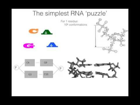
A paper describing Stepwise Monte Carlo's application to a blind prediction of the Zika xrRNA (RNA-Puzzle 18) and several tetraloop-tetraloop receptor interactions, as well as its performance in an extensive 82-motif benchmark, is available at biorxiv.
Modes
By default, the code runs Stepwise Monte Carlo. Applications to RNA loops, mini-proteins, mixed RNA/protein, etc. are not different modes, but instead are defined by input sequences (see below). The code will recognize up to two domains for docking, allowing in principle for ab initio models of RNA-RNA tertiary contacts or RNA-protein interfaces without knowing a priori their rigid body arrangement.
It is possible to run single specified moves given a starting structure, specified through
-move. See Tips below.
Input Files
Required file
You typically will be using two input files:
- The fasta file is a sequence file for all the chains in your full modeling problem. For ease of use, you can specify sequence numbering and chain IDs.
- A pdb file (or set of files) to provide any input starting structures for the problem. Residues in PDB files should have chain and residue numbers that represent their actual values in the full modeling problem.
Optional additional files:
- Native pdb file, if rmsd computation is desired.
- Align pdb file, if one desires to keep the modeling constrained to be close to this structure. [Note that this can be different from the native pdb file, if desired.]
Basic use for structure prediction
A sample command line is the following:
stepwise -fasta 1zih.fasta -s start_helix.pdb -out:file:silent swm_rebuild.outThis assumes that you've set up 1zih.fasta to match, in sequence and numbering, residues 3-10 of 1zih.pdb:
>1zih A:3-10
gcgcaagc
Such a fasta would demand a starting PDB numbered A:3-4 A:9-10 that contains a gc/gc A-form helix.
The code takes about 3 minutes to generate one model, using 50 cycles of stepwise monte carlo. Running more cycles (up to 500) essentially guarantees the solution of this problem, even on a single laptop.
Here's an animation that reaches the known experimental structure.
Additional useful parameters:
The flag -motif_mode is equivalent to -extra_min_res 4 9 -terminal_res 1 12 would ask for the closing base pair of the starting helix to be minimized (but not subject to additions, deletions, or rotamer resampling) during the run, and prevention of residues from stacking on the exterior boundary pair ('terminal res'). It is not obligatory, but allowing relaxation of closing base pairs appears to generally improve convergence in this and other RNA cases.
For RNA cases, -score:rna_torsion_potential RNA11_based_new -chemical::enlarge_H_lj are currently in use to test an updated RNA torsional potential and to help prevent overcompression of RNA helices. These are now turned on by default at the time of publication of the method, after completion of benchmarking.
Design
Design is accomplished simply by specifying n ('unknown nucleotide') in the fasta file instead of a specific sequence at any positions that should be varied.
stepwise -fasta NNNN.fasta -s start_helix.pdb -out:file:silent swm_design.out -cycles 500 -extra_min_res 4 9In contrast to the structure prediction example above, the supplied fasta file includes n to represent unknown nucleotides (an IUPAC standard), but is otherwise identical:
>1zih A:3-10
gcnnnngc
This design strategy generalizes: IUPAC supports ambiguous nucleic acid single letter codes that have been incorporated into Rosetta, as well. Beyond n, Rosetta also supports b, d, h, and v (for 'not a', 'not c', 'not g', and 'not t/u'); r and y (for purines g/a and pyrimidines u/c); w and s (for weak base pairers a/u and strong base pairers g/c); k and m (for keto bases g/u and amine bases a/c).
Note the specification of additional cycles (500 instead of 50). This is necessary to ensure closed, convergent solutions, as the search conformation space is larger in design cases than pure structure prediction cases.
See following demo directory for input files & README:
rosetta/demos/public/stepwise_monte_carlo_rna_loop
Multiple loops
If you have an internal loop motif for an RNA, e.g, two strands connecting two helices, there are two ways to setup the problem.
If you do not know the relative rigid body orientations of the two end helices (this is the typical use case), specify those two chunks in different PDB files.
stepwise -in:file:fasta 1lnt.fasta -s gu_gc_helix.pdb uc_ga_helix.pdb -out:file:silent swm_rebuild.out -extra_min_res 2 15 7 10 -terminal_res 1 8 9 16 -nstruct 20 -cycles 1000 -score:rna_torsion_potential RNA11_based_new -native native_1lnt_RNA.pdb
The starting helices in this case came from the rna_helix application, which is briefly described here. The other new flag here is -terminal_res, which disallows stacking on those residues (its not really necessary here but prevents some silly moves). You'll see nucleotides being added to both helix starts, and eventually merging of the two 'sides' of the problem, as in this movie:
If you do have coordinates for the two end helices (this may happen in loop refinement problems, incl. RNA crystallographic refinement), specify those two chunks in the same PDB file:
stepwise -in:file:fasta 1lnt.fasta -s start_native_1lnt_RNA.pdb -out:file:silent swm_rebuild.out -extra_min_res 2 15 7 10 -terminal_res 1 8 9 16 -nstruct 20 -cycles 1000 -score:rna_torsion_potential RNA11_based_new -native native_1lnt_RNA.pdb
See following demo directory for input files & README:
rosetta/demos/public/stepwise_monte_carlo_rna_multiloop
Protein loops
Protein loops can be handled in a similar way to above RNA cases. [Under the hood, they are treated the same way as RNA.]
An example command line for rebuilding a loop from a starting structure with that loop excised:
stepwise -s noloop_mini_1alc_H.pdb -fasta mini_1alc.fasta -native mini_1alc.pdb -score:weights stepwise/protein/protein_res_level_energy.wts -silent swm_rebuild.out -from_scratch_frequency 0.0 -allow_split_off false -cycles 200 -nstruct 20
Note that most loop modeling problems can be accelerated by cutting out a small 'sub-problem'; this was carried out by hand in the example above, but probably could be set up to happen automatically in Rosetta. Notes on additional flags: -from_scratch_frequency 0.0 -allow_split_off false turn off sampling of dipeptides that can be modeled free and merged into the loop; they are not so useful here, although they don't hurt. Last, not much work has been carried out on the energy function. The protein_res_level_energy.wts weights is an adaptation of score12.wts, as was carried out in this paper.
Input files & demo are in:
rosetta/demos/public/stepwise_monte_carlo_protein_loop
Here's an animation:
One interesting thing to note is that the packing of protein side-chains in stepwise monte carlo uses the new allow_virtual_side_chains setting and a score term free_side_chain that gives a bonus to residues for being virtualized (equal to 0.5 kcal times the number of side-chain torsions). This means that the side-chains only get instantiated if they can pack or form hydrogen bonds, and the results is a rather smoother conformational search.
Mini-proteins built from scratch
For both RNA and proteins stepwise monte carlo can also build models 'from scratch' (this feature will be optimized in the future so that you won't have to build, e.g., RNA helices). An example command line is:
stepwise -fasta rosetta_inputs/2jof.fasta -native rosetta_inputs/2jof.pdb -score:weights stepwise/protein/protein_res_level_energy.wts -silent swm_rebuild.out -cycles 2000 -nstruct 50
Here's an animation of a trajectory that achieves a low energy structure:

Most of the simulation may be spent flickering bits of secondary structure – in the future, we will probably setup some precomputation of these bits so that computation can be focused on build up of the complete mini-protein structure.
Input files & demo are in:
rosetta/demos/public/stepwise_monte_carlo_mini_protein
Tips
What if all the residues are not rebuilt?
If the runs are returning many incomplete and different solutions, increase the number of cycles. If the run returns the same solution over and over again with say, a missing U, stepwise monte carlo is telling you that it thinks that the entropic cost of structuring that nucleotide is not compensated by packing/hydrogen-bonding interactions in any available structural solutions. There are ways to force that bulge to get built (see below) through post-processing.
Running specific moves
It is possible to run single specified moves given a starting structure, specified through -move. This is useful to 'unit test' specific moves, and also serves as a connection to the original stepwise enumeration. In particular, these moves are equivalent to the basic moves in the original stepwise assembly executables (swa_rna_main and swa_protein_main), but can have stochastic sampling of nucleotide/amino-acid conformations to minimize. Furthermore, use of the -enumerate flag recovers the original enumerative behavior. Example in tests/integration/tests/swm_rna_move_two_strands.
Conformational Space Annealing
Conformational space annealing (CSA) is a new population-based optimization for stepwise monte carlo. When running stepwise with CSA, each job knows the name of a silent file with a "bank" of models and updates it after doing some monte carlo steps. Each model in the bank has a "cycles" column (and its name is S_N, where N = cycles). This is the total number of cycles in the CSA calculation over all jobs completed at the time the model is saved to disk. Currently, decisions to replace models with "nearby" models are based on RMSD. The RMSD cutoff can be set via the -csa_rmsd option.
The following parameters define the amount of computation performed by stepwise with CSA:
Rosetta options:
-cycles                               number of monte carlo cycles per update (default: 50)
-nstruct                              number of updates per structure in bank (default: 20)
-csa_bank_size                        number of structures stored in the bank (default: 0)


Compute per job:
total cycles  = <cycles> * <nstruct>

Total Compute:
total cycles  = <cycles> * <nstruct> * <csa_bank_size>
To run stepwise with CSA, create a README_SWM with the following command-line:
stepwise @flags -cycles <cycles> -nstruct <nstruct> -csa_bank_size <csa_bank_size>To setup the jobs on a cluster, run the following command:
rosetta\_submit.py README\_SWM SWM <njobs> <nhours>csa_bank_size should match njobs, the number of cores running in parallel.
What do the scores mean?
The score terms are similar to those in the standard Rosetta energy functions for protein or RNA (which themselves may be unified soon). For completeness, some additional terms relevant for stepwise applications are described here.
***Energy interpreter for silent output:
score                                            Final total score
fa_atr                                           Lennard-jones attractive between atoms in different residues
fa_rep                                           Lennard-jones repulsive between atoms in different residues
fa_intra_rep                                     Lennard-jones repulsive between atoms in the same residue
lk_nonpolar                                      Lazaridis-karplus solvation energy, over nonpolar atoms
hbond_sr_bb_sc                                   Backbone-sidechain hbonds close in primary sequence (i,i+1)
hbond_lr_bb_sc                                   Backbone-sidechain hbonds distant in primary sequence
hbond_sc                                         Sidechain-sidechain hydrogen bond energy
geom_sol_fast                                    Geometric solvation energy for polar atoms (environment-independent)
loop_close                                       Entropic cost for loops not yet instantiated but whose endpoints are fixed
ref                                              Cost for instantiation of a full RNA/protein residue, backbone + sidechain
free_suite                                       Bonus for freeing a terminal phosphate or sugar (may be unified with ref)
free_2HOprime                                    Bonus for freeing a 2'-OH hydroxyl (may be unified with ref)
intermol                                         Cost of bringing two chains together at 1 M (-conc flag can change this)
other_pose                                       Score of sister poses (if building off separate PDBs, prior to merge)
linear_chainbreak                                Closure term to keep chainbreaks together upon loop closure
atom\_pair\_constraint                             any pairwise distance constraints (not implemented yet)
coordinate\_constraint                            any constraints to put atoms at specific coordinates (not implemented yet)

[RNA stuff]
fa\_elec\_rna\_phos\_phos                            Distance-dep. dielectric Coulomb repulsion term between phosphates
rna\_torsion                                      RNA torsional potential.
rna\_sugar\_close                                  Distance/angle constraints to keep riboses as closed rings.
fa\_stack                                         Extra van der Waals attraction for nucleobases, projected along base normal
stack\_elec                                       Electrostatics for nucleobase atoms, projected along base normal.

[protein stuff]
pro\_close                                        Distance/angle constraints to keep prolines as closed rings.
fa\_pair                                          Lo-res propensity for protein side-chains to be near each other
hbond\_\*                                          Other h-bond terms, probably will all get unified
dslf\_\*                                           Disulfide geometry terms, unified in later score functions
rama                                             Score for phi/psi backbone combination
omega                                            Tether of protein backbone omega to 0° or 180°
fa\_dun                                           Protein side chain energy
p\_aa\_pp                                          -log P( aa | phi, psi ), enters into current bayesian formalism for score
free\_side\_chain                                  bonus (of 0.5 * nchi) for virtualizing a protein side chain

[Following are provided if the user gives a native structure for reference]
missing                                          number of residues not yet built in the structure
rms                                              all-heavy-atom RMSD to the native structure of built residues.
Post Processing
Finishing the 'full model'
The stepwise application is not guaranteed to finish construction of the entire full modeling problem in the number of cycles provided. We would like to obtain models that have all residues fully represented, as doing so satisfies two requirements:
- Pragmatically speaking, clustering methods often require the models being clustered to have the same length
- The
stepwiseapplication computes two measures of RMSD to native, neither of which is likely exactly what you want or expect.-
rmsis computed only over built residues, so a simulation that builds precisely one of ten residues will probably have a very goodrmsdespite being very far from the full modeling problem desired. -
rms_fillis computed by imagining that the remaining residues in the problem are all in A-form backbone conformations extending from each exposed connection. This is quick to compute at the end of a modeling problem and helps to penalize largely-unbuilt models.
-
We would like to fill in these models with 'unfolded' residues, and we do so using the application build_full_model. This application runs in two principal modes, each of which eexcutes the same top-level plan -- to place all the residues from the intended full modeling problem and compute a realistic RMSD, as well as base-pairing statistics to evaluate how much of the native structure's key features were recovered.
The application always takes a silent file through -in:file:silent and outputs one via -out:file:silent. In one mode, run with -virtualize_built true -caleb_legacy true, we install virtual residues one at a time with stepwise moves. This is very fast, perhaps seconds per structure. The second (-fragment_assembly_mode true) installs all residues at once, as 'repulsive-only' variants (that experience only van der Waals repulsion and chain-closure penalties) and then uses the fragment assembly code to optimize its conformation. This method takes considerably more time and isn't deterministic but does have the advantage of producing conformations of self-avoiding chains. (In theory, the virtual residues installed by the first mode could self-intersect.) A standard command line used in the Watkins, 2018 paper is:
build_full_model.linuxclangrelease –in:file:silent swm_rebuild.out –in:file:fasta t_loop_modified_fixed.fasta –out:file:silent swm_rebuild_full_model.out –in:file:native t_loop_modified_fixed_NATIVE_1ehz.pdb –stepwise:monte_carlo:from_scratch_frequency 0.0 –out:overwrite true –score:weights stepwise/rna/rna_res_level_energy4.wts –virtualize_built false –fragment_assembly_mode true –rna:evaluate_base_pairs true –superimpose_over_all true –allow_complex_loop_graph trueSubsequently, we can take resulting models and run them through a clusterer to analyze how well the run converged on low-RMSD solutions.
Extraction Of Models Into PDB Format
The models from the above run are stored in compressed format in files like swm_rebuild.out You can see the models in PDB format with the conversion command.
extract_pdbs -in:file:silent swm_rebuild.outExperimental stuff
Lo-res mode

In this mode, created by the flags -lores seeks to enable tests of stepwise with way more cycles than allowed above. Instead of minimizing, the model is optimized by 100 cycles of fragment assembly after each stepwise add/delete/resample, in a low resolution scorefunction (here, rna_lores.wts supplemented with loop_close and ref). Leads to over-optimization of an inaccurate function in most loop modeling or motif cases, or worse optimization than classic FARFAR setup for loops. Contact Rhiju if you're interested in trying on more complex cases, where there might be a 'win'.
Variable-length loop mode
This is a generalization of stepwise design where loops (specified as strings of n in the FASTA file) are allowed to change their length during the run. Maximum loop lengths are based on FASTA file. Run stepwise with -vary_loop_length_frequency 0.2 to check it out -- contact Rhiju to make this robust, and to optimize predicted delta-G for tertiary folding by comparison to free energies from the Vienna RNA package.
New things since last release
This is a new executable as of 2014, with continuing updates to end of 2018.
See Also
- Applications for deterministic stepwise assembly:
- Overview of Stepwise classes
- Developer's internal documentation for Stepwise (for developers)
- Structure prediction applications: Includes links to these and other applications for loop modeling
- RNA applications: Applications to be used with RNA or RNA and proteins
- RosettaScripts: The RosettaScripts home page
- Application Documentation: List of Rosetta applications
- Running Rosetta with options: Instructions for running Rosetta executables.
- Comparing structures: Essay on comparing structures
- Analyzing Results: Tips for analyzing results generated using Rosetta
- Solving a Biological Problem: Guide to approaching biological problems using Rosetta
- Commands collection: A list of example command lines for running Rosetta executable files
- RiboKit: RNA modeling & analysis packages maintained by the Das Lab